⚡️ 🌀 ⚡️ 🌀 ⚡️
      ∰∭∬⫘⫘⫘∬∭∰
  ⎛∿∿∿∿⎞|░▒▓█▓▒░|⎛∿∿∿∿⎞
  ⌇|◣◢❂◣◢|⫯∑∑∑⫯|◣◢❂◣◢|⌇
   ⎪⎨⎬⎨⎬⎨⎬⎪ ☯️ ⎪⎨⎬⎨⎬⎨⎬⎪
  ⌇|◥◤∞◥◤|⫰∏∏∏⫰|◥◤∞◥◤|⌇
  ⎝≈≈≈≈⎠|░▒▓█▓▒░|⎝≈≈≈≈⎠
       ∯∮∳⫘⫘⫘∳∮∯
       ⚡️ 🌀 ⚡️ 🌀 ⚡️

Some months ago I read the book “Active Inference - The Free Energy Principle in Mind, Brain, and Behavior” by Thomas Parr, Giovanni Pezzulo, and Karl J. Friston. I found it to be a good introduction for the Free Energy Principle (FEP) and Active Inference. The following text is a short and hand-waved recapitulation of some of the main ideas exposed there. At the end, I add some thoughts and references to its relevance and relation to reinforcement learning.

The free energy principle made too simple

A simple (but not too simple) explanation of the FEP may be found here, but, honestly, it’s way too “unsimple” for this, so here’s my attempt to explain it… simply.

To formulate the FEP the founding question should probably be “what is a thing?”, and for this question to have any sense we must assume that a “thing” is separable from anything that is not that thing (i.e. its environment). Thinking probabilistically, a way to define this separability is to take the collection of variables that make the thing statistically independent from its environment, conditional on the information of those variables. That is, such variables mediate the interactions between the the thing and its environment. This concept comes from statistics/ML and is called a Markov blanket.

My main man Markov

Now - the word thing could have a connotation for “objectness”, but the thing need not be an object – it could be something less concrete, as long as we can define its Markov blanket and separate it from its environment. As such, it might be more adequate to use the word system. That way we could refer to biological, computer, social systems, etc. We could take this even further and question whether this separation needs to be stationary or unique. This is in itself a pretty deep rabbit-hole that can get frogs blocked on X, so let’s keep it as simple as possible.

We may call the variables pertaining to the system itself their internal states and the variables pertaining to its environment as the external states, whereas the variables of the actual separation are its blanket states.

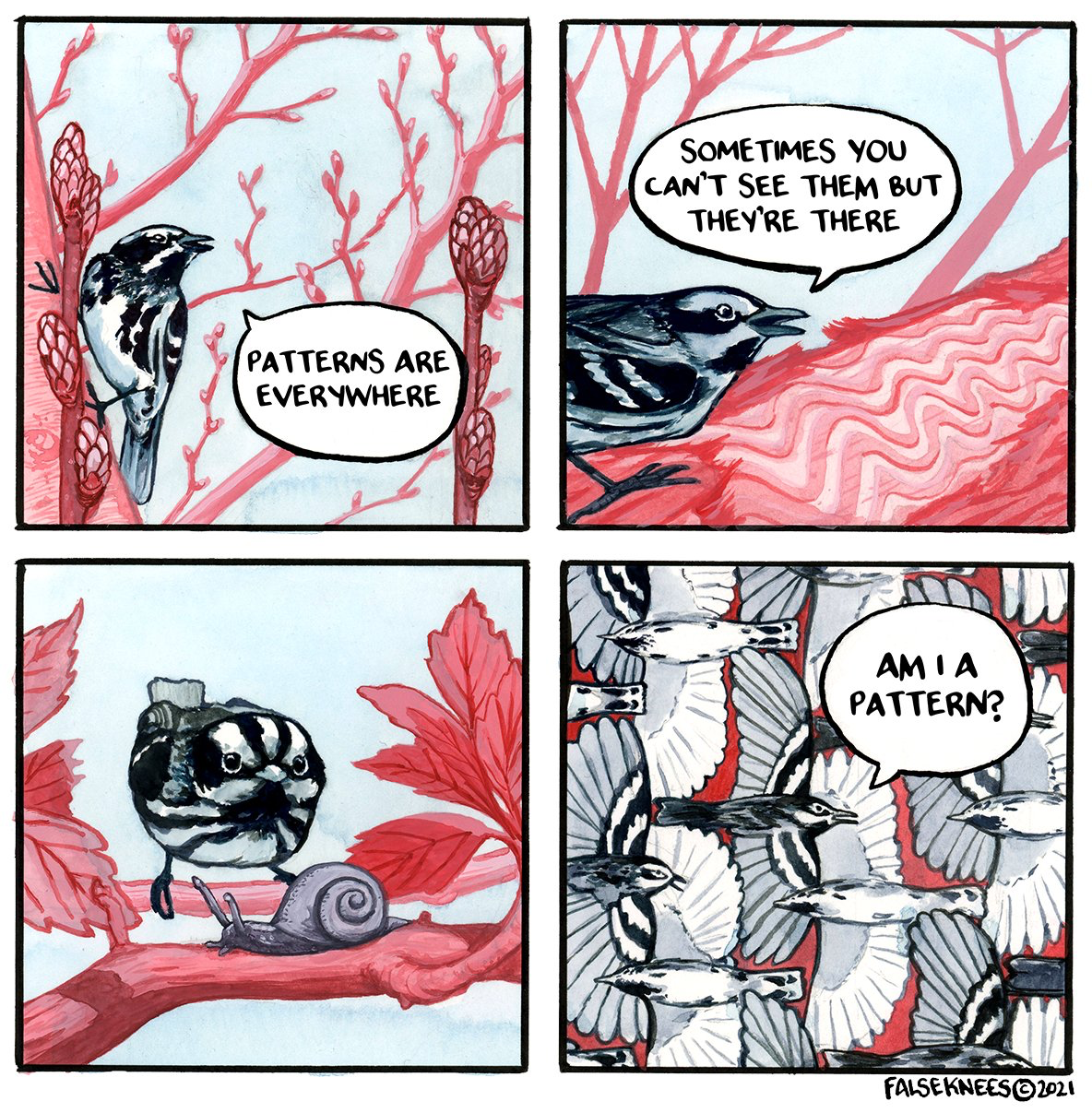
Image credit: False Knees

So far so good! We may imagine many boundaries :) but what’s the point? Why care about the boundary of a cloud? Of my body? Of my self? Well… the second law of thermodynamics roughly states that, in a closed system, the total entropy will never decrease over time. This entails that if we draw boundaries on arbitrary “systems” that are passive, it might well be that these systems could “give in” to entropy (that is, degrade, break-down ☠️). We would be much more interested in drawing boundaries around systems that persist over time 🌱 That is, we care about systems that adapt themselves to interact to its environment to resist this entropic force.

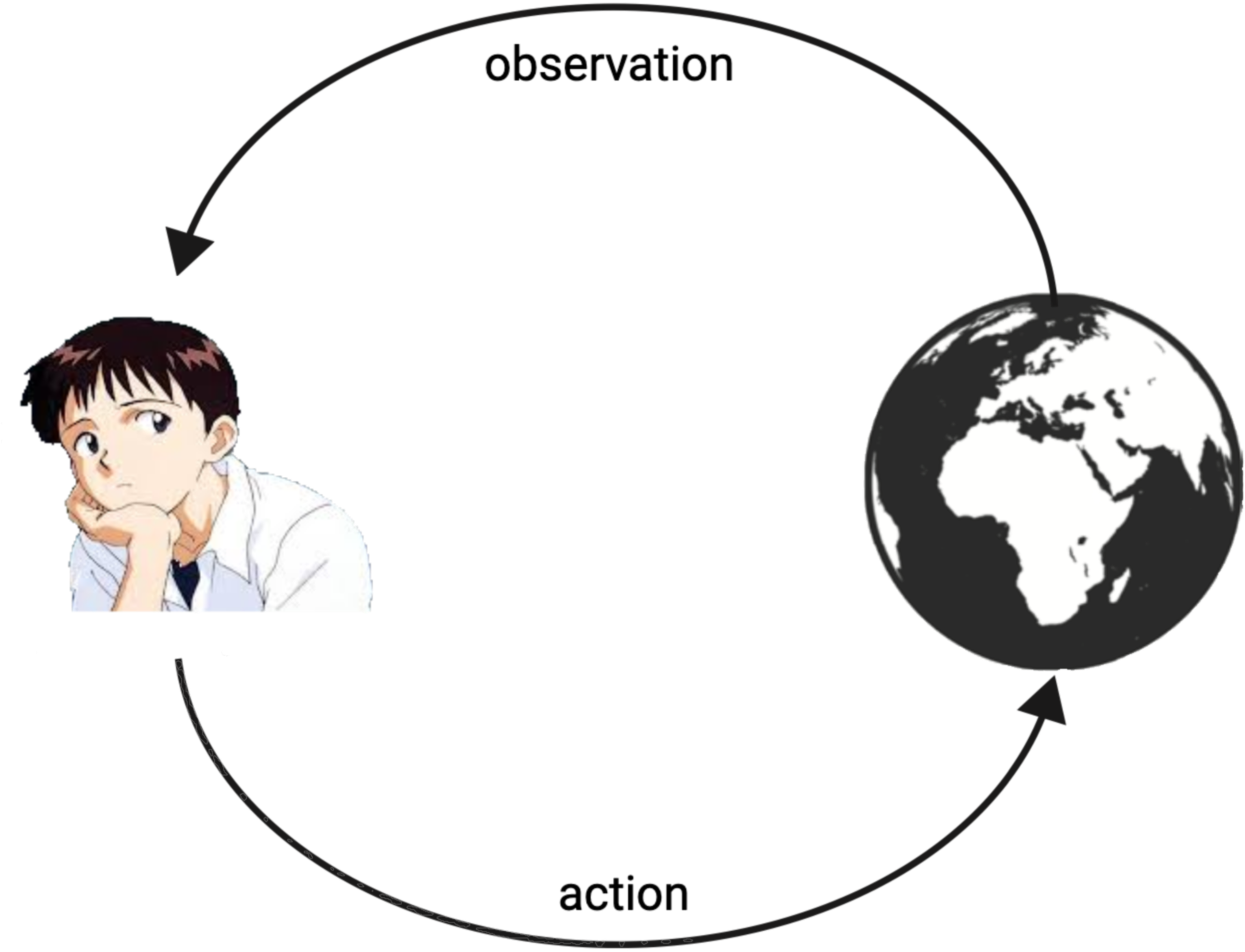
Keeping this in mind, the FEP borrows¹ from the concept of a Markov blanket to conceptualize this separation between system and its environment, and it goes further into a more functionally segregated question: what types of separation might there be between a system that effectively persists over time and its environment? Arguably, there are two: actions and observations; that is, states through which a system can influence its environment, and states through which a system is influenced by its environment. So, we end-up with an action-perception loop similar to what we see in reinforcement learning and other fields. We may call these special systems agents.

These specific agentic systems minimize entropy – by the very definition of what we’re interested in – and in doing so what they achieve is to stay within the bounds that allow their persistence in time, which we may call “self-evidencing”. This is a concept common to many fields. For instance, from a physiological perspective this is essentially the idea of homeostasis or from a more general perspective in cybernetics there’s the concepts of autopoiesis.

To understand why there’s this equivalence between entropy minimization and self-evidencing, we should note that Shannon entropy is, by definition, the average surprise, which is the negative log-evidence. Suppose \(y\) are the observed states by a given system. Following the notation from the book:

That is, the entropy of the distribution over the states, \(P(y)\), is equal to the expected value of the surprise under the distribution \(P(y)\), where the surprise, \(S(y)\), is defined as \(-lnP(y)\). This means that it is equivalent to minimize entropy and to increase the “model evidence” (likelihood), \(P(y)\), which can be thought of as achieving a higher probability on those preferred states. For example, think of this as trying to maximize the probability that your core body temperature is within the normal physiological range.

But exactly how might a system stay within its desired bounds? Well, we already mentioned it is via its Markov blanket partitioned into both observation and action. That is, a system regulates its environment to minimize surprise, and, thus, resist entropy. In order to do this, the system must first model its environment. In cybernetics, this is known as the “good regulator theorem”.

This is arguably very intuitive! Imagine you have to keep things under control in any given context. How would you go about that if you don’t even have an idea of what the context is or how it develops!? To expand on this, imagine that the state of the environment is a variable, \(x^*\). Then, the joint distribution of this state and the observations, \(y\), form a joint distribution, \(P(x^*, y)\). This is basically the generative process of the environment; that is, how the environment generates data. Although the agent does not know the underlying dynamics of the environment, by the good regulator theorem, it must at least have a model of it. This model may be expressed as \(P(x, y)\), where \(x\) are not necessarily the true states of the environment, but at least hypotheses over those states. To infer \(x\) from \(y\) – which is to compute \(P(x \mid y)\) – is precisely the task that an agent would be concerned with. It’s easy to think of this in the context of a card game, like blackjack. In that case you don’t know the underlying state (\(x\)) of the deck of cards (the environment) and you only observe (\(y\)) the cards that have been dealt. Yet, if you want to win (observe your desired states) you should probably have at least some idea or approximation (i.e. a hypothesis of the state of the cards, \(x\)) so that you can chose what to do (ie. hit, stand, double-down, etc.).

So now we have two things we are trying to keep in mind: first, the surprise over the observed states of the agent, and, second, the generative model of the environment. But there’s a couple of problems here. For starters, \(x^*\) (the true state of the environment), may not even be accessible to the agent, as we have mentioned. Furthermore, computing \(P(x \mid y)\) might be intractable or even infeasible. The most natural assumption would be that agents somehow approximate the posterior, so we use a proxy distribution, \(Q(x)\), and a metric, such as the KL divergence, between such proxy distribution and the true model posterior \(P(x \mid y)\) :

Thus, keeping in mind this approximation, what an agent would be doing, really, is to minimize the approximation error of to the posterior, and maximize the model log-evidence, which is the following:

The previous equation can be rearranged as follows:

The above is defined as the free energy, and it implies that if the agent minimizes this, it doesn’t have to calculate the posterior anymore, it only needs the joint distribution \(P(x,y)\) (i.e. its generative model).

This has two other equivalent formulations, which can help with intuition.

The first one would be to form the expression as the sum between an energy term and an entropy term:

The name energy makes reference to the homonymous term in the Helmholtz free energy formulation, but it may be more intuitively interpreted as the consistency between the approximation \(Q(x)\) and the generative model \(P(x,y)\). On the other hand, the entropy term pushes the approximation to have more uncertainty. This can be interpreted as saying that whenever observations are scarce, using an approximation over the states of the environment that is maximally entropic would be optimal. In other words, when we know little of the environment, we can assign the same probabilities to all of its states!

The second formulation would be as follows:

Here, the first term can be thought of as a complexity term, which measures how far is the approximate posterior from the priors over \(x\). The second term is the accuracy of the approximation. This formulation is akin to model selection (i.e. choosing models that are minimally complex but that also accurately account for data).

With these re-formulations in mind, we can see that the FEP provides an elegant and concise way to theorize about systems that resist entropic forces, but, thus far, we haven’t even incorporated action into the equations. Indeed, we mentioned that the agent wants to achieve both preferable states, and a regulation of its environment via a model of it, but the FEP seems static, or at least, retrospective, in the sense that it focuses on present observations. How might it be extended into the future? This is where action comes in.

The step towards active inference

Active inference is the extension of the FEP to make sense of streams of observations/states into the future, and, as such, it has a prospective nature, shedding a light into planning and decision-making.

Instead of a single state \(x\) and a single observation \(y\), let’s now consider a stream \(\bar{x}\) of states of the environment, and a stream of observations, \(\bar{y}\). Of course, these streams should be thought of in the context of a stream of actions (i.e. a policy), \(\pi\).

Using the FEP equations above, but with this prospective focus, and omiting the conditional on the policy \(\pi\), for simplicity, we would get the following expression:

where

So what has changed? To start with, we now have actions in the model. The system’s actions influence its environment, and the stream of current + future observations will influence present actions. This means that, whereas the free energy is dependent on the observations, here we have a dependency on the policy, \(\pi\) , which, in turn, conditions the probability of the future observations!

The above may be re-written as:

This is, of course, very similar to the second reformulation of the free energy in the previous section. The difference is that now the second term is an expectation over the entropy of the distribution of future observations, given the future states. This leads to a different interpretation of the expression. It now can be thought of as a value composed of a risk part in the first term, and an expected ambiguity in the second term. In other words, minimizing this value entails reducing the risk, which can be interpreted as the expected complexity cost of the approximation, and reducing the expected uncertainty, which is essentially the expected inaccuracy.

Having said this, something we might consider is to switch the focus of the first term (the risk term) from states to observations. Why would this make sense? Well, mostly because sometimes the state-space is unknown, and it is more intuitive to think of preferences over outcomes/observations². With this in mind, we get the following inequality:

The expression on the right-hand can have an analogous interpretation, and it can also be re-written as:

The above is the expected free energy. The first term can be interpreted as the information gain – i.e. how much information about the states \(\bar{x}\) is brought in by the stream of observations \(\bar{y}\), which can be measured as the KL divergence between the distributions over \(\bar{x}\), when conditioning on \(\bar{y}\) vs when we don’t :) This means that agents choose policies that induce observations that carry more information with them. For example, imagine a situation where you need to go to the dentist. If you had a good recall of your schedule, having a look at your calendar will not give you any new information – indeed, you might as well just call and book your appointment. However, normally, you would first take a look at your calendar to resolve the uncertainty around your schedule. Such step would allow you to gain enough information to then successfully achieve your goal to go to the dentist.

The second term of the expected free energy can be thought as utility maximisation, or the “exploitation” of policies that lead to preferrable observations. Thus, to minimise expected free energy it would be necessary not only to seek policies that induce “exploration” or information gain, but also to seek those that confirm priors over preferred states.

To conclude, the concept of the expected free energy extends the idea of the free energy principle over future time-horizons, and in particular sets a useful theoretical framework to reason about planning and exploration.

Active inference vs reinforcement learning

For anyone relatively familiar with the (perhaps more widely known) ideas of reinforcement learning, the concepts treated in active inference might seem really familiar.

Indeed, there are no substantial practical difference between the two. Reinforcement learning is formalized with the concept of a Markov decision process (MDP).

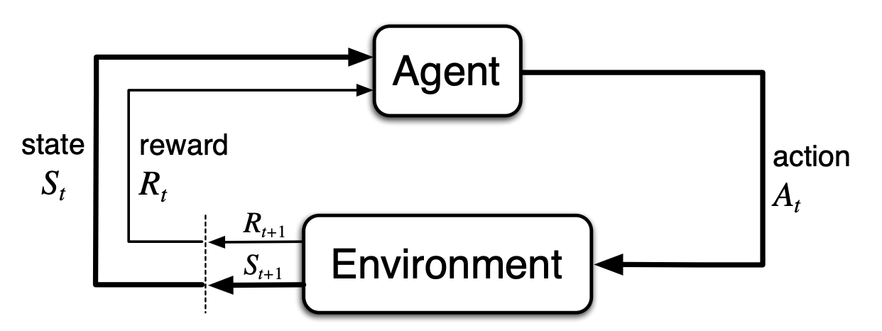
MDP diagram taken from Reinforcement Learning: An Introduction by Sutton & Barto

An important component of MDPs are rewards. In active inference, rewards are implicitly encoded as probability distributions over the observations – as we mentioned, agents want to reach their desired states. However, this does not entail a fundamental change. If anything, maybe reinforcment learning can be seen as a subset of active inference. A deeper discussion about this topic may be found in this paper.

Furthermore, the exploratory aspect we mentioned in the previous sections is not unique to the active inference framework. In reinforcement learning, for example, exploration bonuses may be added; again, this shows that there is no significant difference between the two, insofar as practical advantages go. For technical details on this, this is a good reference. Also, a more general overview of some of these points may be found in Beren’s Retrospecive on Active Inference.

Final thoughts

The FEP and the active inference framework seem to be, at least in my opinion, a cool theoretical framework to think about agency. However, I do think that most of what makes it look appealing is this facade of it having the potential to be one of those “theories of everything”. So, after reading Parr et al’s book, I stand inspired by the ideas, but dubious about its general applicability, and, especially after having also explored Beren’s work, I’m doubtful that it provides any edge over the traditional RL methods in practical use-cases. I’ll remain open to learning more about the FEP and active inference, especially given my lack of knowledge in neuroscience, but remain unconvinced it’s some sort of panacea, at least in the context of AI, as some tend to claim.

🍀